In one-factor ANOVA, we normally treat one independent variable on the dependent measured variable. In factorial ANOVA, we increase the number of factors from one to see not only the impact of each individual factor, but also more importantly draw conclusion about the interaction effect of all the factors
Factorial design or experiment addresses on testing the effect of multiple factors (independent variables) on the dependent variable
| Factor B | |||||
| Factor A | Level 1 | Level 2 | … Level j | ||
| Level 1 | Cell 11 | Cell 12 | Cell 1j | ||
| Level 2 | Cell 21 | Cell 22 | Cell 2j | ||
| … Level k | Cell k1 | Cell k2 | Cell kj | ||
From the above table, each factor is divided into its possible combinations (factorial)
Let us take an example of 2 x 2 factorial ANOVA test where each independent variable has two possible levels. Suppose we want to study student test scores in certain university. The university offers two class sessions. One in the morning and another in the evening. The university also offers two teaching modes for each session. Online teaching and in-class teaching. In this case we have two factors or independent variable. Class session is factor A while teaching mode is factor B
In factorial ANOVA we want to test the interaction effect of both factor A and factor B as well as individual effects of either factor A or factor B
To conduct the experiment two students are randomly selected for each cell in the table above. For example we test two students in cell 11, another two students in cell 12 an so on. In ANOVA terminology we say we replicated each cell of the table above with two subjects
Our example is summarized in the table below along with test scores of the replications
| Teaching mode | |||
| Class session | In-class | Online | |
| Morning | 67 71 | 58 65 | |
| Evening | 71 73 | 66 70 |
From this table, we have total of 8 experimental units while replication per treatment is 2
Now the interaction question is
“Do some students in one teaching mode score better in one class session while other students in different teaching mode score better in another class session?”
To test the hypothesis, we will use F – distribution by calculating the F – statistic
To understand how to calculate the F-statistic for factor A, factor B and the interaction factor, we first need to have the following formulas

The term

Is called MSE (mean square due to error)
The above formula looks totally confusing and lengthy. To simplify it let calculate F-statistic for factor A levels
We break down the formula as below

Factor A mean can be calculated as
| Morning | Mean11 = (67+71)/2 = 69 | Mean12 = (58+65)/2 = 61.5 | Total mean = (69+61.5)/2 = 65.25 |
| Evening | Mean21 = (71+73)/2 = 72 | Mean22 = (66+70)/2 = 68 | Total mean = (72+68)/2 = 70 |
Factor B mean can be calculated as
| In-class | Online |
| Mean11 = (67+71)/2 = 69 | Mean12 = (58+65)/2 = 61.5 |
| Mean21 = (71+73)/2 = 72 | Mean22 = (66+70)/2 = 68 |
| Total mean = (69+72)/2 = 70.5 | Total mean = (61.5+68)/2 = 64.75 |
Overall mean = (65.25 + 70 + 70.5 + 64.75)/4 = 67.625
Now we continue working on the remaining parts of the above F formula

Now we compute variance of factor A. As an example level 1 (morning) cells (11 and 12)
| x | ||||
| 67 | 65.25 | 1.75 | 3.0625 | 1.02 |
| 71 | 65.25 | 5.75 | 33.0625 | 11.02 |
| 58 | 65.25 | -7.25 | 52.5625 | 17.52 |
| 65 | 65.25 | -0.25 | 0.0625 | 0.021 |
| Variance = 29.581 |
Similarly variance of factor A level 2 (evening) is 8.67
Next we calculate the MSE to finalize the calculation of the F-statistic

Now the F-statistic is

Hence the F-statistic due to factor A only is 4.718.
You see how the computation of factor A only is tedious. You are still required to compute F-statistic for factor B and the interaction of both factor A and B
Hence it is recommended to use computer statistical software to analyze the factorial or two-way ANOVA. In our case we will use SPSS as follows
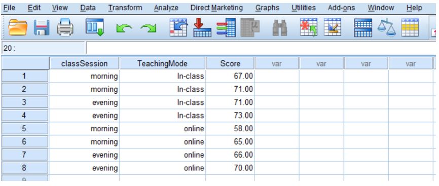
First step is data entry as shown below. We create for the two independent variables and the dependent variables
Next go to analyze > General linear models > Univariate to pop up the Univariate dialog box
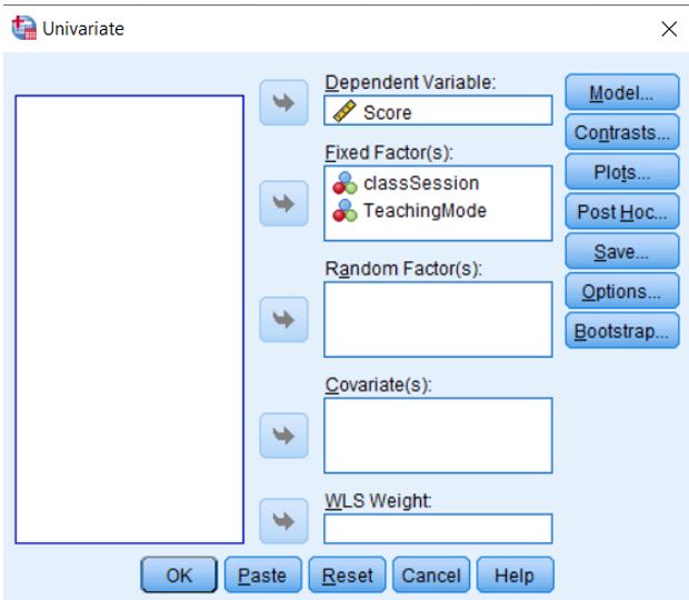
Once everything is setup as shown above, click ok to generate the following results dialog box
| Between-Subjects Factors | |||
| Value Label | N | ||
| classSession | 1.00 | morning | 4 |
| 2.00 | evening | 4 | |
| TeachingMode | 1.00 | In-class | 4 |
| 2.00 | online | 4 |
| Tests of Between-Subjects Effects | |||||
| Dependent Variable: Score | |||||
| Source | Type III Sum of Squares | df | Mean Square | F | Sig. |
| Corrected Model | 117.375a | 3 | 39.125 | 3.682 | .120 |
| Intercept | 36585.125 | 1 | 36585.125 | 3443.306 | .000 |
| 45.125 | 1 | 45.125 | 4.247 | .108 | |
| TeachingMode | 66.125 | 1 | 66.125 | 6.224 | .067 |
| classSession * TeachingMode | 6.125 | 1 | 6.125 | .576 | .490 |
| Error | 42.500 | 4 | 10.625 | ||
| Total | 36745.000 | 8 | |||
| Corrected Total | 159.875 | 7 | |||
| a. R Squared = .734 (Adjusted R Squared = .535) |
The final part is interpretation of the tests between subjects effects table
- The p-value of the classSession factor is greater than the test significance (0.108 > 0.05). Hence we accept the null hypothesis that the two class session shown no score difference
- The p-value of the TeachingMode factor is greater than the test significance (0.067 > 0.05). Hence we accept the null hypothesis and conclude that there is no statistical evidence showing the two teaching modes produce different student scores
- The p-value of the interaction is greater than the test significance (0.490 > 0.05). Hence there is not difference of student scores in once class session and teaching mode than those in another class session and teaching mode

